Caustics in Large-Scale Structure
Back to research
Catastrophe Theory
Though the title is daunting, I'm not going to propose the end of the world.
Actually, this theory studies the sudden changes of the characteristics of a system when changing certain variables.
This is similar to phase changes in regular matter, for instance when water turns to ice by changing its temperature.
On this page, I will describe how I use this theory to classify gravitational collapse and structure formation on the largest scales, analogous to phase changes.
In general, these points of sudden change are called singularities, and the type of change is named its catastrophe.
One can determine these singularities by following the potential function of the system, the function which determines its behavior.
At the times when the derivative of the potential is zero, you can find its singularities.
More commonly in calculus, these points are referred to as the function's critical points.
However, the singularities we care about are often degenerate, meaning that higher derivatives are zero as well, and represent a dramatic change in the system's characteristics.
Now that we have the basic idea, let's explore Lagrangian catastrophe theory, which is where we will discover caustics later on.
In this framework, we use simulations to study an evolving fluid, like dark matter (DM), in Lagrangian space.
That is, at the start of the simulation, we assign each DM particle, \(i\), a coordinate, \(\mathbf{q}_i\), relative to the particles around it, that doesn't change with time.
This coordinate signifies that particle's starting position.
Then, for each particle, subtracting the Lagrangian coordinate from its Eulerian coordinate \(\mathbf{x}(t,\mathbf{q}_i)\), or its true position in space at time \(t\), yields its displacement: \(\mathbf{x}(t, \mathbf{q}_i)= \mathbf{q}_i + \mathbf{s}(t, \mathbf{q}_i)\).
Note that each particle has the same mass, and the start of the simulation spreads them out in a nearly constant density, with tiny fluctuations to represent quantum randomness imprinted into the initial conditions of the universe.
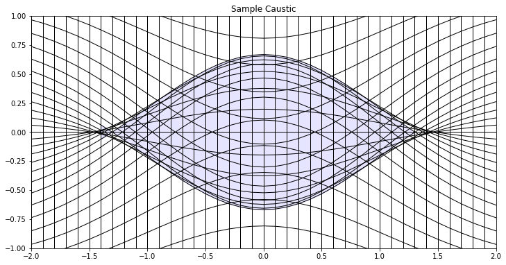
Fig. 1: A caustic with a vertically-varying potential function; the shaded region is a "fold" catastrophe, while the boundary is a "cusp" catastrophe

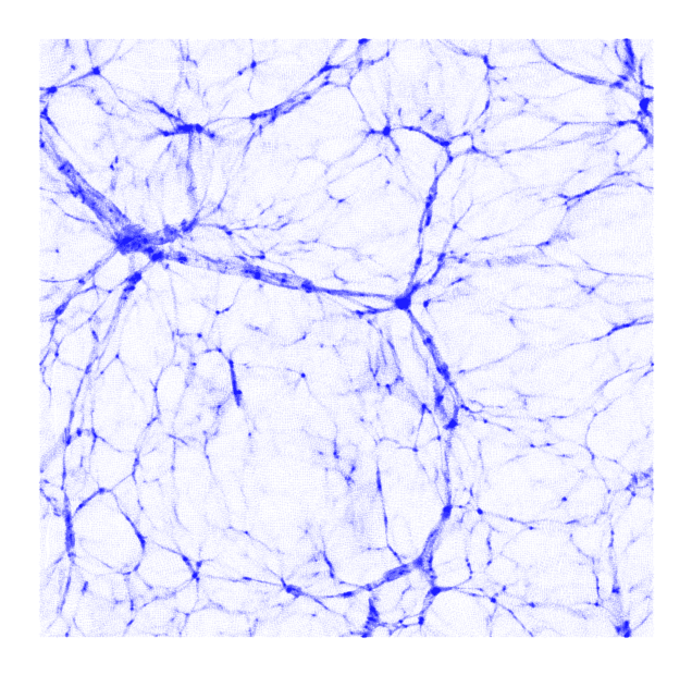
Fig. 2: Initial distribution of a dark matter simulation with slight fluctuations, and its later evolution
Caustics
Let's not lose the objective we set out to accomplish.
I promised that all this can be used to understand gravitational collapse.
In fact, the displacements are all we need to construct what we call caustics, which are simply the singularities corresponding to Lagrangian catastrophes.
Explicitly, caustics trace out surfaces containing multi-stream regions.
A single multi-stream point in Eulerian space corresponds to several single-stream points in Lagrangian space.
In simple terms, this means that DM particles which started at different coordinates overlap on one coordinate.
Recalling that caustics are the boundaries of the multi-stream regions, we can deduce that they mark regions with infinite density, infinitessimal radius, and thus finite mass.
To go about evaluating these caustics, we calculate the gradients of the displacements, which return the deformation tensor, or the matrix describing how the fluid deforms and shifts.
(A more complete picture of the math involved can be found in this paper.
Here I am more focused on the intuition and idea behind the process.)
Taking the determinant of the deformation tensor yields a measure of how the volume changed at each point in space, with 1 as no change, >1 corresponding to a growth, and <1 to a shrink.
A value of 0 is therefore what we are looking for, as it is linked to a shrink down to an infinitessimal volume.
Finally, negative values correspond to a mirror flip across an axis.
To simplify, let's take an example.
Suppose we track the evolution of the determinant over time for a single DM particle named "Bob".
Refer to figure 3 for the example, as it corresponds to an actual particle in the simulation I used.
The determinant must start at 1, as it represents no change to the volume surrounding Bob.
In a region where gravity leads to collapse, the determinant must decrease, as the space around Bob gets smaller.
Eventually, Bob encounters other particles, such as "Alice", reaching a determinant of 0.
Bob and Alice occupying the same space thus form a multi-stream region.
But they don't just stop there, they continue traveling past each other.
As such, the determinant crosses zero and becomes negative, and this event is called shell-crossing.
Note that in a cosmic void, the determinant likely never crosses zero, and may even increase above 1.
Every particle in the simulation whose determinant crosses zero gets to be part of a caustic.
Then plotting all the caustics in the simulation allows for a reliable tracer of the cosmic web.
Such a gif is displayed in figure 4, where I show the IllustrisTNG DM simulation at z=1.
Since the only information we needed to construct and analyze the caustics was the displacements, we successfully developed a parameter-free identifier of the cosmic web.
But the technique is more powerful than this.
In fact, using catastrophe theory, we can classify the type of structure within the web based on how many times the determinant crosses zero (and other more complicated conditions, such as the eigenvectors of the deformation tensor).
These classes have names, and often physical interpretations:
- \(A_2\): Fold catastrophe. Corresponds to a simple collapsed region.
- \(A_3\): Cusp catastrophe. Corresponds to a wall.
- \(A_4\): Swallowtail catastrophe. Corresponds to a filament.
- \(A_5\): Butterfly catastrophe. Corresponds to a cluster.
- \(B_4\): Hyperbolic catastrophe. Corresponds to a different type of filament.
- \(B_5\): Parabolic catastrophe. Corresponds to a different type of cluster.
Now that we have such a unique, parameter-free analysis tool of the cosmic web, it is natural to connect it to my previous project on using persistent homology, as that is also purely geometric. Rather than using subhalos as the data points representative of cosmic structure, we can use caustics. In particular, mapping the caustics with the times of first shell-crossing outputs figure 5. It is plotted in Lagrangian coordinates, or the initial position space, which is why it is a 256 by 256 grid since the simulation itself began with \(256^3\) particles. The brighter spots are regions which experienced gravitational collapse earlier in the simulation, while the majority dark area denotes particles which have never done so. Using a superlevel filtration (as opposed to the previously-explored distance filtration), we can run persistent homology and analyze patterns in the cosmic web.
This is the next phase of my project, and will be discussed in greater detail once I have results. Thanks for reading!
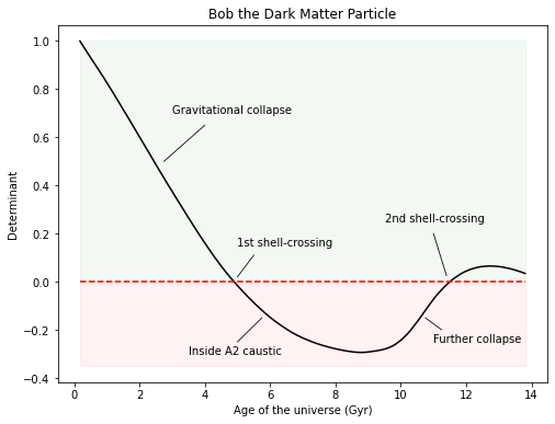
Fig. 3: Bob's caustic formation journey
Fig. 4: Caustics in a simulation; blues are DM particles, rainbows are caustics; axes are in units of Mpc
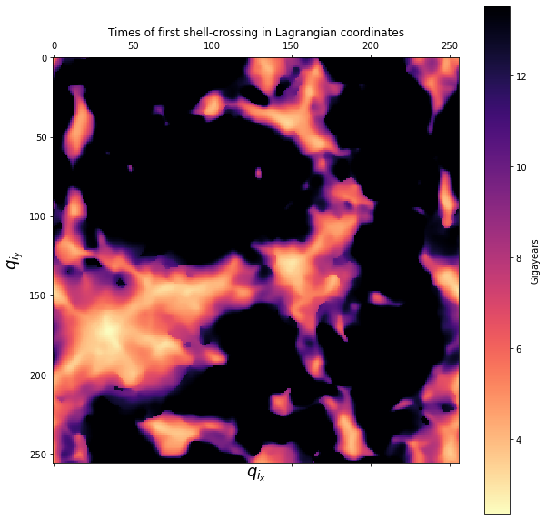
Fig. 5: The times of first shell-crossing for a thin slice of a simulation in Lagrangian coordinates