Astrophysics Background

In our universe, matter organizes itself on the largest scales into one connected structure known as the cosmic web. This web is made of smaller sub-structures known as walls, filaments, and nodes, each of which connect to each other to create web-like patterns. Between these structures lie cosmic voids, which I have studied in more detail here. Each of these phenomena are part of a field within cosmology focusing on the creation and evolution of large-scale structure on the megaparsec scale, and studying these can help us understand the origins of the universe and how it might continue to evolve.

An example of such structures can be seen on the figure on the right. This image is taken from a thin slice in the middle of a dark matter simulation from the IllustrisTNG collection. The simulation spans a volume of 35 x 35 x 35 Mpc³, and the slice is about 0.7 Mpc wide. It is a snapshot at a redshift of about z=1.

Note that I will be using co-moving Mpc, and to convert to "real" distances, one needs to multiply this by the dimensionless Hubble constant used by IllustrisTNG, h=0.677.

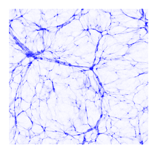
Fig. 1: the cosmic web in a simulation

Persistent Homology

In order to study the cosmic web and its "connectedness" mathematically, it is useful to employ the techniques of persistent homology. This tool has been used in the fields of neuroscience, materials science, and even nuclear collisions. Here I will give a very brief overview for the "physicist's" persistent homology.

In the context of cosmology, topology studies the shape and connectivity of a structure. As my colleague Georg Wilding put it, it defines distance not in terms of a specific metric, "but by a notion of neighbourhood or adjacency." This implies that even physically distant objects in the universe can be considered "connected" through some path or network that links their two positions, effectively making them neighbors. The types of distinguishable networks these structures form are associated with their homology. This quantifies the space through the amounts and dimensionalities of holes.

For example, one might expect that a hollow sphere has no holes. Indeed, in the layman sense, an unpunctured, perfect sphere will not allow you to put a chain through to lock your bike, like a torus might have. However, this is only referring to the one-dimensional hole, which is the type of hole that is enclosed by tracing a one-dimensional curve on a surface. There are other types of holes, namely the two-dimensional hole, which the sphere does exhibit. This hole is enclosed by a two-dimensional surface in a three-dimensional space, and can be called a cavity.

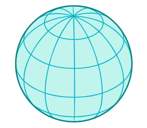
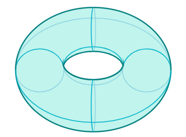
Fig. 2: a hollow sphere and a hollow torus

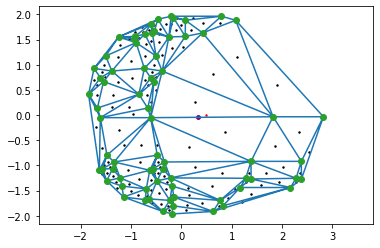
Computing these holes based on different filtrations, or thresholds of separations, is the essence of persistent homology. Filtrations can be set on any piece of information one might like, such as a distance or local density. An example of a distance-based filtration can be observed in the figure to the right.

This is a set of points in a two-dimensional space. Around each point is a blue circle of equal radii, representing the distance filtration. Whenever the associated circles of two different points overlap, they are connected by a red line. Three lines and three points connected together trace a triangle. Each of these structures is a type of simplex, or the n-dimensional generalization of a triangle. For instance, the 0-dimensional simplex is a point, the 1-dimensional simplex is a line, then a triangle (2-simplex), a tetrahedron (3-simplex), a pentachoron (4-simplex), and so on. Connected simplices are said to be part of a simplicial complex.

Simplicial complexes, such as the one in the figure, can represent interesting and quantifiable structures. Using the distance filtration, one can start with a low distance value (small circles) and increase it gradually, keeping track of when two circles overlap and connect two points together. When enough points connect to form a loop, it is considered a cycle and its birth time is recorded. Cycles that are only comprised of triangles are not significant and are therefore not considered to ever be born. In this example, a birth time is not really a time, but corresponds to the length of the longest line segment in a cycle at the moment a hole is enclosed, as that is the last line segment to have been created. As the filtration continues to increase, more points connect to each other, until the former cycle is only comprised of triangles. The moment this happens, the shape is considered to be dead and its death time is recorded.

The birth and death times can be plotted on a persistence diagram such as the one in figure 4. In the example, there are two cycles, one much larger than the other. I am able to count the number of cycles by simply counting the number of non-simplex (non-triangle) holes. We expect the larger cycle to take longer to die, since the circles need to increase to a sufficient radius to overlap with circles on the other side Thus, we find two points on the diagram corresponding to the two cycles.

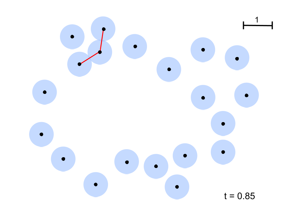
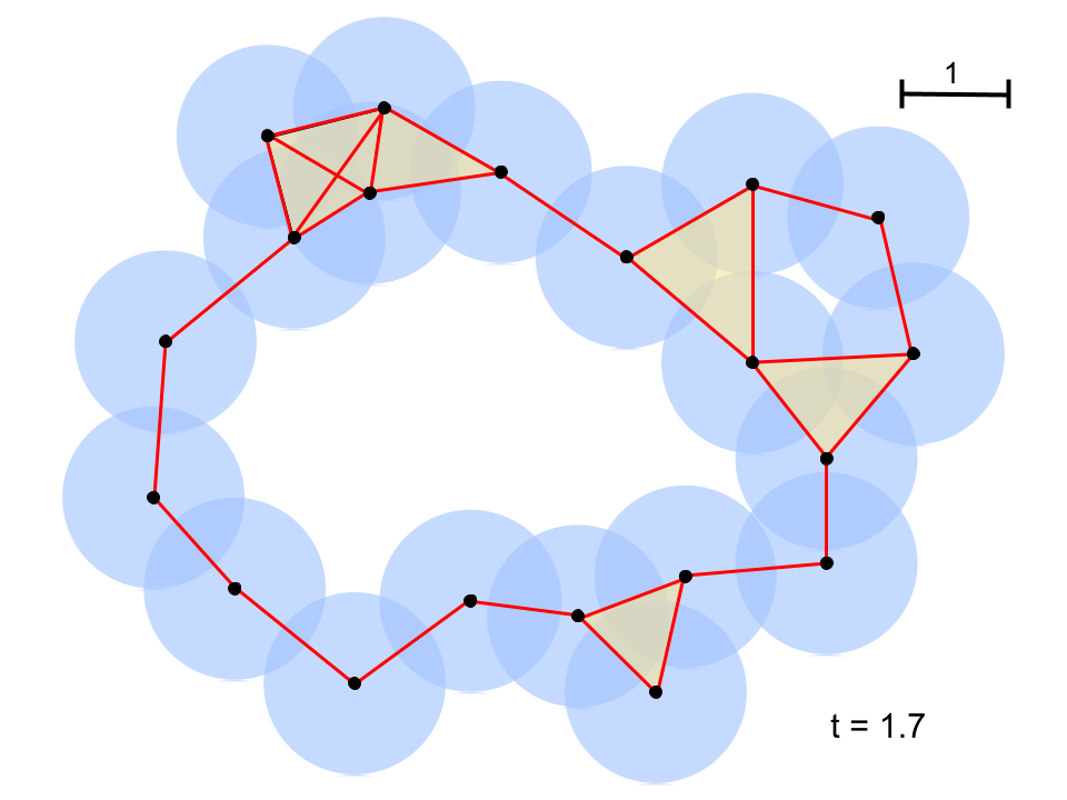
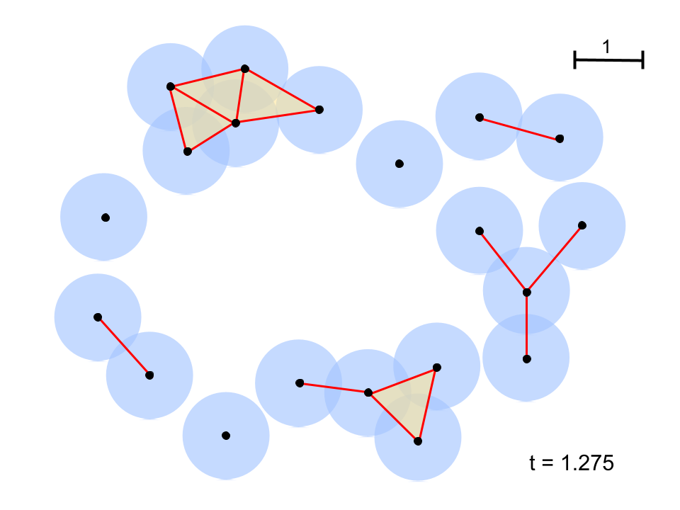
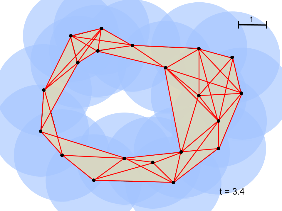
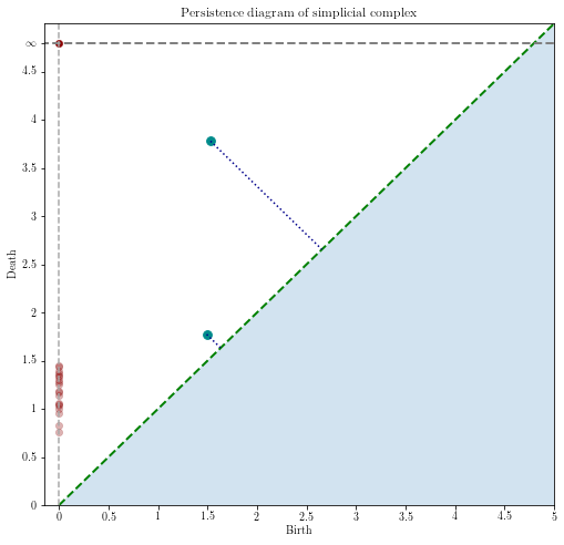
Fig. 4: a persistence diagram corresponding to the simplicial complex

Indeed, they are born around the same time, but one dies much sooner while the other persists. One can define the persistence of a feature by its distance to the diagonal. A point of low persistence is close to the diagonal, while a point of high persistence is farther away. Importantly, points cannot be found under the diagonal, since that corresponds to a feature dying before it is born. Finally, the red points on the left side correspond to the times at which connections are made between "islands" of points, merging from two separate complexes to one. The point at infinity indicates that the last time more than one complex was present was at a value of just under 1.5, and no new complex islands were found, even at an infinite distance filtration.

There are several important strengths of persistence diagrams when trying to quantify the connectedness of data. First, it allows for the reduction of a complex dataset to its basic topological features, emphasizing those which the human eye can agree with. Second, it is robust against noise, and any slight wiggles in the positions of the points in the example would yield a very similar persistence diagram. Third, it can be used to understand underlying structure of a dataset beyond just its largest features.

In the next section I will describe how I applied persistent homology to the cosmic web, and suggest some future research questions.

Cosmic persistence

A natural place to start is to notice the regularity of structure in figure 1. In order to characterize the connectedness of the cosmic web, a tracer needs to be chosen. That is, data that accurately and faithfully represents the distribution of matter. My idea for this project was to make use of information provided by IllustrisTNG itself, which is the mass halos and their corresponding subhalos. These are simply the galaxy clusters and their constituent galaxies, but including their dark matter contents. I chose the central subhalo of each halo as its representative.

Figure 5 shows two copies of a thin 31.5 Mpc slice of the 205 Mpc simulation, with only the main subhalos plotted. The second slice highlights voids detected by persistent homology. It is able to idenify the holes in this slice by tracing the encompassing loops with a distance-based filtration, as before. Three of the loops with high persistence are identified by red, green, and magenta. These are, of course, not the only detected voids, but let's take these as prominent examples. Visually, it is clear that the loops surround an area which is mostly empty. It may not be entirely empty because though the slice is thin, there is still some depth in the image and those points may be located in the foreground or background.

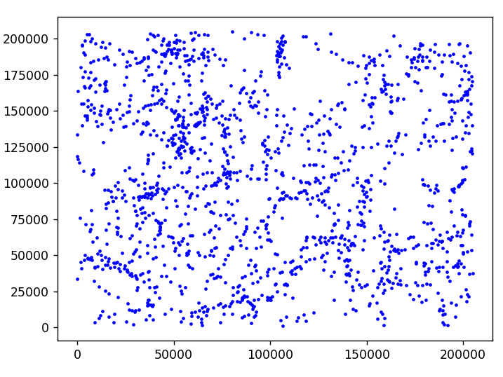
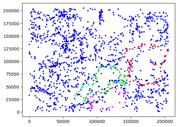
Fig. 5: A 31.5 Mpc slice of the simulation, with and without the detected voids

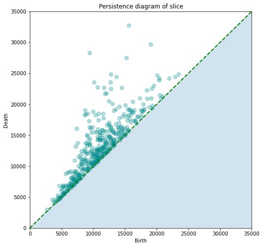
Fig. 6: The associated peristence diagram of the slice, representing 1-dimensional loops

In addition, some lone galaxies may inhabit voids anyways. Furthermore, the voids appear to be bordering each other, ignoring the "noise" that separates them. This is promising, and is indicative of the algorithm working as intended, picking out loops and voids, and assigning each one its birth and death times.

Okay, But What's Next?

Now that we have an understanding of the toolset, we can move on to bigger and better things. There are a lot of possible questions to answer, but the ones I tackled in my research involve cosmic voids. In the next page, I will move on from 1-dimensional holes to 2-dimensional cavities, and discover the true power of persistent homology. Click the image to the right to go to voids!

---

Back to top